📗 Explanation · understanding-oriented

Temporal Dynamics in Visual Processing

This document explains the concept of temporal dynamics in visual processing and how DynVision implements these dynamics in recurrent neural networks.

Introduction

Visual processing in biological systems is not instantaneous. Rather, it unfolds over time, with neural activity evolving continuously through complex interactions between feedforward, recurrent, and feedback connections. This temporal dimension of visual processing is often overlooked in standard deep learning models but is crucial for understanding many aspects of biological vision.

DynVision focuses on implementing these temporal dynamics in artificial neural networks, enabling models that better capture the time-dependent properties of biological visual systems.

Temporal Processing in Biological Vision

The Time Course of Visual Processing

When light hits the retina, it triggers a cascade of neural activity that propagates through the visual system:

1. Photoreceptors: Convert light into electrochemical signals (~10-20ms)
2. Retinal Processing: Initial processing in the retina (~20-30ms)
3. LGN Relay: Thalamic relay to cortex (~5-10ms)
4. V1 Response: Primary visual cortex activation (~40-60ms after stimulus)
5. Higher Cortical Areas: Subsequent activation of V2, V4, IT (~60-120ms)
6. Feedback Signals: Recurrent processing within and between areas (~100-300ms)

This creates a complex temporal pattern of activity, with information flowing both forward and backward through the system.

Key Temporal Phenomena

Several important temporal phenomena characterize biological visual processing:

1. Response Latencies

Different visual areas respond with characteristic latencies:

• V1: ~40-60ms
• V2: ~50-70ms
• V4: ~60-80ms
• IT: ~80-120ms

These latencies reflect not just the time required for signals to propagate but also the processing time within each area.

2. Temporal Summation

Neural responses don't simply follow the temporal profile of the stimulus. Instead, they exhibit:

• Integration: Responses to longer stimuli increase up to a point (temporal summation)
• Subadditivity: The increase is sublinear, eventually saturating
• Persistence: Activity continues briefly after stimulus offset

3. Adaptation

With sustained or repeated stimulation, neural responses typically decrease:

• Fast adaptation: Rapid decrease during continuous stimulation
• Repetition suppression: Reduced response to a repeated stimulus
• Recovery: Gradual recovery with longer intervals between stimuli

4. Contrast-Dependent Timing

The timing of neural responses depends on stimulus contrast:

• Higher contrast → Faster response onset
• Higher contrast → Earlier peak response
• Higher contrast → More transient response

5. Rhythmic Activity

Neural activity often shows oscillatory patterns:

• Alpha rhythms (~8-12Hz)
• Gamma oscillations (~30-80Hz)
• Theta rhythms (~4-8Hz)

These oscillations may coordinate activity across different brain regions and contribute to attention and perception.

Implementing Temporal Dynamics in DynVision

DynVision implements several key components to capture these temporal dynamics:

1. Continuous-Time Dynamical Systems

Unlike traditional discrete-time recurrent neural networks, DynVision models neural dynamics using a continuous-time differential equation where heterogeneous connectivity and delays interact over a single time constant \(\tau\):

\[ \begin{align} &{\color{#c4380f}\tau} \frac{d{\color{#18359c}r}}{d{\color{#5f5b5b}t}} = -{\color{#18359c}r}({\color{#5f5b5b}t}) + {\color{#821ca9}\Phi} {\color{#821ca9}\bigl[} {\color{#41960e}I}({\color{#5f5b5b}t}) + {\color{#17a89c}J}{\color{#18359c}r}({\color{#5f5b5b}t}) {\color{#821ca9}\bigr]} + {\color{#556B2F}B}\\[4pt] &{\color{#18359c}r_l}({\color{#5f5b5b}t}) = {\color{#18359c}r_l}({\color{#5f5b5b}t}-{\color{#b8621a}dt}) + \frac{{\color{#b8621a}dt}}{\color{#c4380f}\tau} \Bigl( -{\color{#18359c}r_l}({\color{#5f5b5b}t}-{\color{#b8621a}dt}) + {\color{#821ca9}\Phi} {\color{#821ca9}\bigl[} {\color{#41960e}I_l}({\color{#5f5b5b}t}-{\color{#b8621a}dt}) + \textstyle\sum{\color{#17a89c}J_l}\,{\color{#18359c}r(\cdot)} {\color{#821ca9}\bigr]} + {\color{#556B2F}B_l} \Bigr)\\[4pt] &\sum_{{\color{#5f5b5b}s}=0}^{{\color{#5f5b5b}t}-{\color{#b8621a}dt}} {\color{#17a89c}J_l} {\color{#18359c}r}({\color{#5f5b5b}s}) = {\color{#17a89c}J_{FF}}\!\cdot\!{\color{#18359c}r_{l-1}}({\color{#5f5b5b}t}-{\color{#b8621a}\Delta_{FF}}) \;+\; {\color{#17a89c}J_{RC}}\!\cdot\!{\color{#18359c}r_l}({\color{#5f5b5b}t}-{\color{#b8621a}\Delta_{RC}}) \;+\; {\color{#17a89c}J_{FB}}\!\cdot\!{\color{#18359c}r_{>l}}({\color{#5f5b5b}t}-{\color{#b8621a}\Delta_{FB}}) \;+\; {\color{#17a89c}J_{SK}}\!\cdot\!{\color{#18359c}r_{<l-1}}({\color{#5f5b5b}t}-{\color{#b8621a}\Delta_{SK}}) \end{align} \]

Where the colors denote: ● \(\tau\) — dynamical timescale · ● \(r\) — network activations · ● \(I\) — external input · ● \(B\) — bias · ● \(t\), \(s\) — time dimension · ● \(\Phi\) — activation function · ● \(J\) — network connectivity · ● \(dt\), \(\Delta\) — time step / delays

What this shows:

1. Differential equation — network activity \(r\) evolves continuously over time \(t\) with a dynamical timescale \(\tau\), driven by external input \(I\) and modulated by recurrent connectivity \(J\), then passed through a nonlinearity \(\Phi\) with an additive bias \(B\).

2. Euler discretization — a numerical stepwise approximation for layer \(l\) at the next time step \(t\). The Euler method advances the activity by \(dt/\tau\) times the difference between the driven state (inside the brackets) and the current activity.

3. Heterogeneous connectivity — the sum over all connections to layer \(l\) separates into four biologically motivated pathways: feedforward (\(J_{FF}\), from the preceding layer), lateral recurrent (\(J_{RC}\), within the same layer), feedback (\(J_{FB}\), from higher layers), and skip (\(J_{SK}\), from earlier non‑adjacent layers). Each pathway has its own delay \(\Delta\) (an integer multiple of \(dt\)), matching cortical propagation distances.

This formulation provides several advantages:

• More biologically realistic temporal evolution
• Smoother dynamics with appropriate time constants
• Explicit modeling of integration, decay, and heterogeneous delays
• All connection types operate within a single unified dynamical system

2. Numerical Solvers

To implement these continuous dynamics computationally, DynVision uses numerical solvers:

Euler Method

The simplest solver, which approximates the solution using:

\[x(t+dt) = x(t) + \frac{dt}{\tau} \cdot [-x(t) + W(x(t))]\]

This method is computationally efficient but may require small timesteps for accuracy.

3. Biologically Motivated Delays

DynVision implements different delays for different connection types (\(\Delta_{FF}\), \(\Delta_{RC}\), \(\Delta_{SK}\), \(\Delta_{FB}\)). Each delay is an integer multiple of the integration step dt:

• Feedforward delay (\(\Delta_{FF}\)): 0 ms in the default engineering-time unrolling; set to a positive value (e.g. 10 ms) for biological-time unrolling.

• Recurrent delay (\(\Delta_{RC}\)): 6 ms by default, independent of the unrolling convention.

• Skip / feedback delays (\(\Delta_{SK}\), \(\Delta_{FB}\)): adjusted automatically when converting between engineering and biological time.

These delays approximate signal-propagation times in biological systems, where feedforward connections involve longer-range projections and recurrent connections involve shorter-range lateral interactions. The choice of engineering vs. biological time only shifts responses in time; it does not change the dynamics (see Engineering vs. Biological Time).

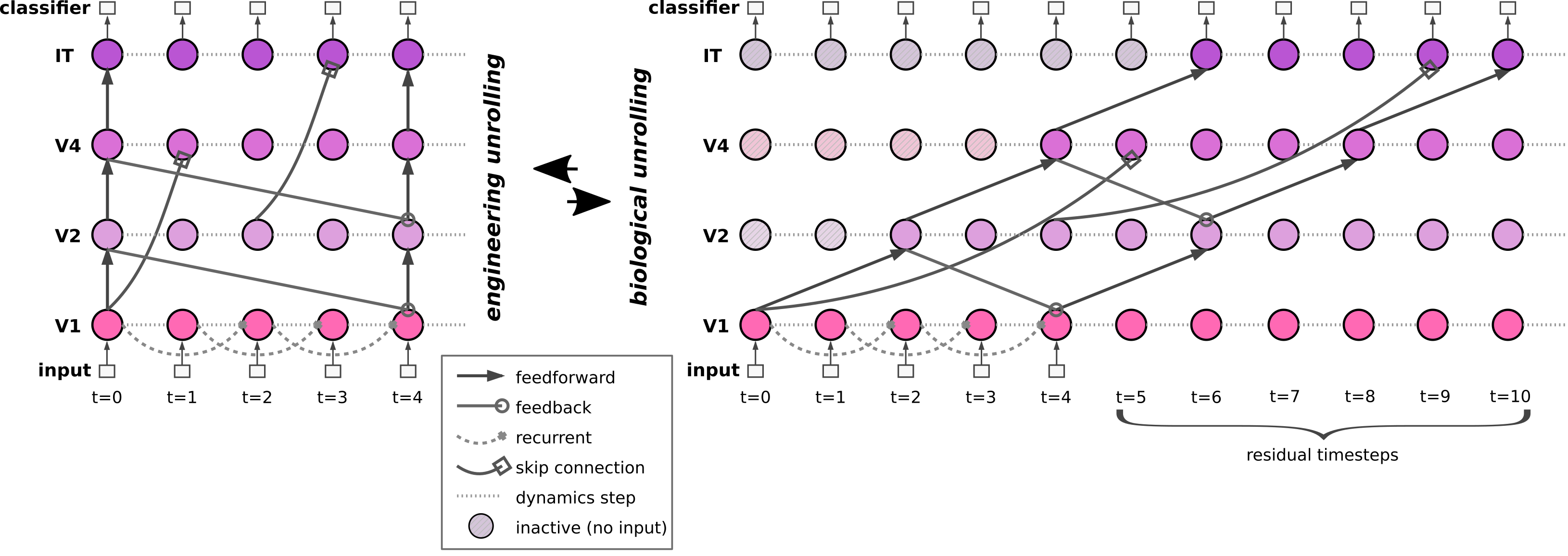
Figure: The same recurrent network can be unrolled in engineering time (left, all delays collapsed) or biological time (right, delays match cortical propagation distances). The toolbox automatically converts between these conventions.

4. Time Constants

The time constant \(\tau\) governs how quickly a layer's activity tracks its driven state. The DynVision default is \(\tau = 5\) ms (see the default training configuration). Larger \(\tau\) values produce slower rise and decay; transient onset overshoots (also seen in cortical responses) appear only for small \(\tau\) (\(< 9\) ms).

DynVision allows setting the time constant per layer, enabling layer-specific temporal dynamics. As a rough orientation:

• Fast time constants (~5-10 ms): rapid response components
• Medium time constants (~20-50 ms): sustained responses
• Slow time constants (~100-500 ms): adaptation and integration

5. Specialized Data Loaders

To test temporal dynamics, DynVision provides specialized data loaders:

• StimulusDuration: Presents stimuli for varying durations
• StimulusInterval: Presents repeated stimuli with varying intervals
• StimulusContrast: Presents stimuli at different contrast levels

These loaders create temporal stimulus patterns that probe specific aspects of temporal processing.

Relationship to Biological Phenomena

DynVision's implementation of temporal dynamics allows it to capture several key biological phenomena:

Response Latencies

By using feedforward delays and layer-specific time constants, DynVision models show latency progressions similar to biological systems. These latencies emerge naturally from the model's architecture and dynamics, without explicit training.

Temporal Summation

The dynamical systems formulation naturally produces subadditive temporal summation:

1. With short stimuli, responses increase linearly with duration
2. With longer stimuli, responses saturate due to:
3. Balance between excitation and decay
4. Recurrent inhibitory connections
5. Neural adaptation mechanisms

This matches the pattern observed in biological neurons, where responses don't simply track stimulus duration.

Adaptation and Recovery

DynVision models show adaptation to sustained or repeated stimuli:

1. During sustained stimulation:

   • Initial strong response
   • Gradual decrease over time
   • Eventual steady-state response

2. For repeated stimuli:

   • Strong response to first presentation
   • Reduced response to second presentation
   • Recovery with longer intervals

These adaptation patterns emerge from the interaction between recurrent connections and neural dynamics.

Contrast-Dependent Timing

The models also show contrast-dependent response timing:

1. Higher contrast → Faster response onset
2. Higher contrast → Earlier peak response

This emerges from the interaction between input strength and the threshold dynamics in the neural equations.

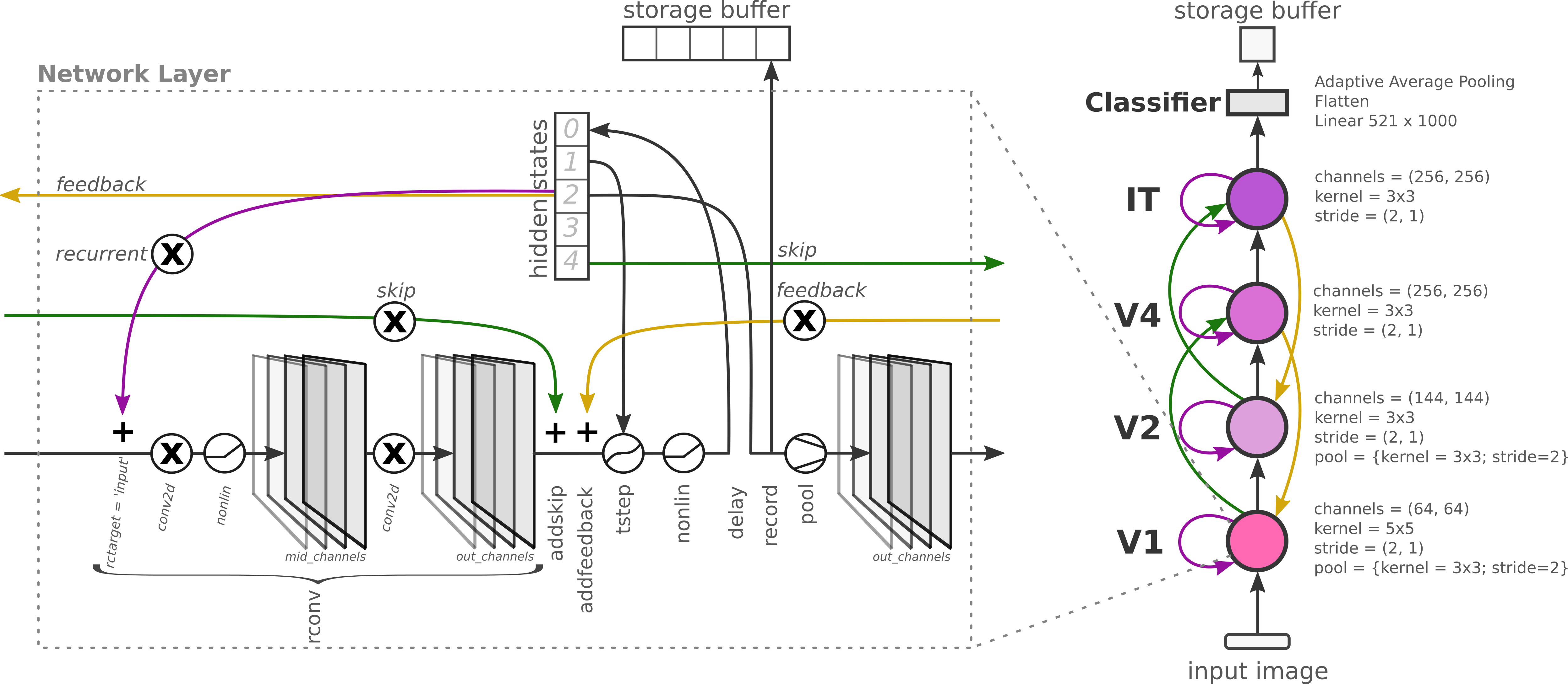
Figure: The RCNN architecture showing the configurable ordering of operations within each layer (convolution → bias → dynamics step → nonlinearity → pooling) that determines where in the neuron activation sequence recurrent signals are integrated.

Empirical Validation

DynVision models have been validated against electrophysiological recordings from human visual cortex (Groen et al., 2022). The key finding is that different recurrent configurations give rise to functionally distinct dynamic regimes:

1. Temporal normalization regime — Models with full lateral recurrence targeting the layer output, combined with strong activity-loss regularization, naturally produce adaptation (reduced response to repeated stimuli), sublinear temporal summation, and contrast‑dependent response timing. This happens without any explicit divisive‑normalization operation; the recurrent weights converge to effectively inhibitory values that stabilize feedforward activity.

2. Noise-robustness regime — A different configuration with full recurrence targeting the middle of a layer's computations, trained with minimal activity‑loss on purely static images, produces substantially improved robustness to Gaussian noise (approaching human‑level performance curves from Jang et al., 2021) but shows weaker temporal normalization.

The two regimes thus dissociate: the activity loss that promotes biologically realistic temporal normalization also reduces noise robustness, while middle‑target recurrence enhances denoising at the cost of weaker temporal normalization. This suggests that recurrence serves functionally distinct roles depending on architectural context.

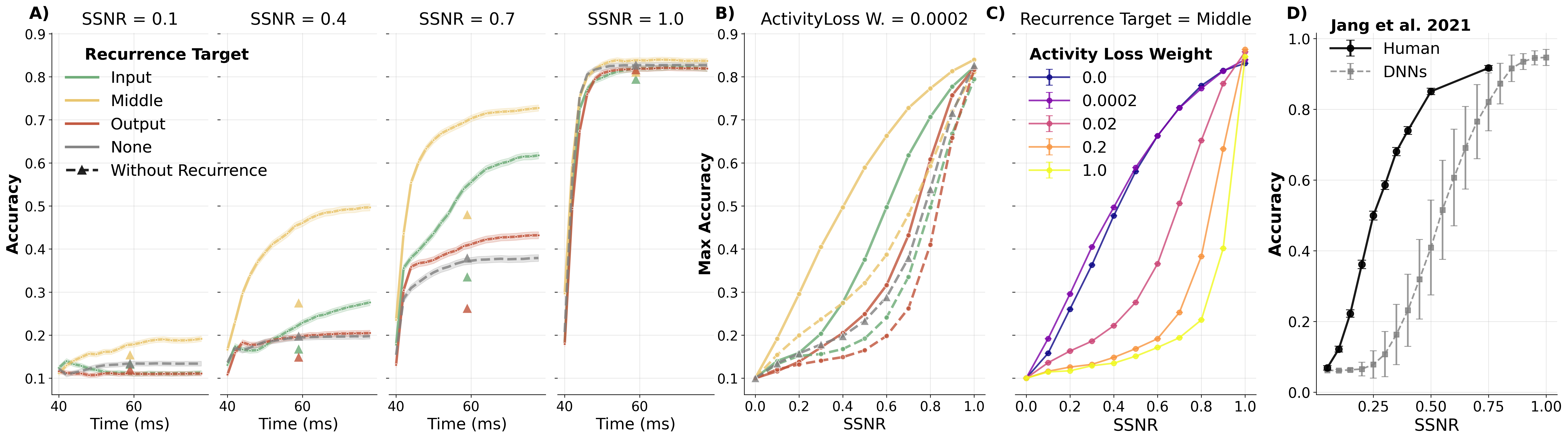
Figure: systematic comparison of model performance across recurrence targets (left vs center panels), demonstrating that the location where recurrent signals are integrated (pre- vs post-activation) qualitatively changes the learned dynamics.

Temporal Parameters in Detail

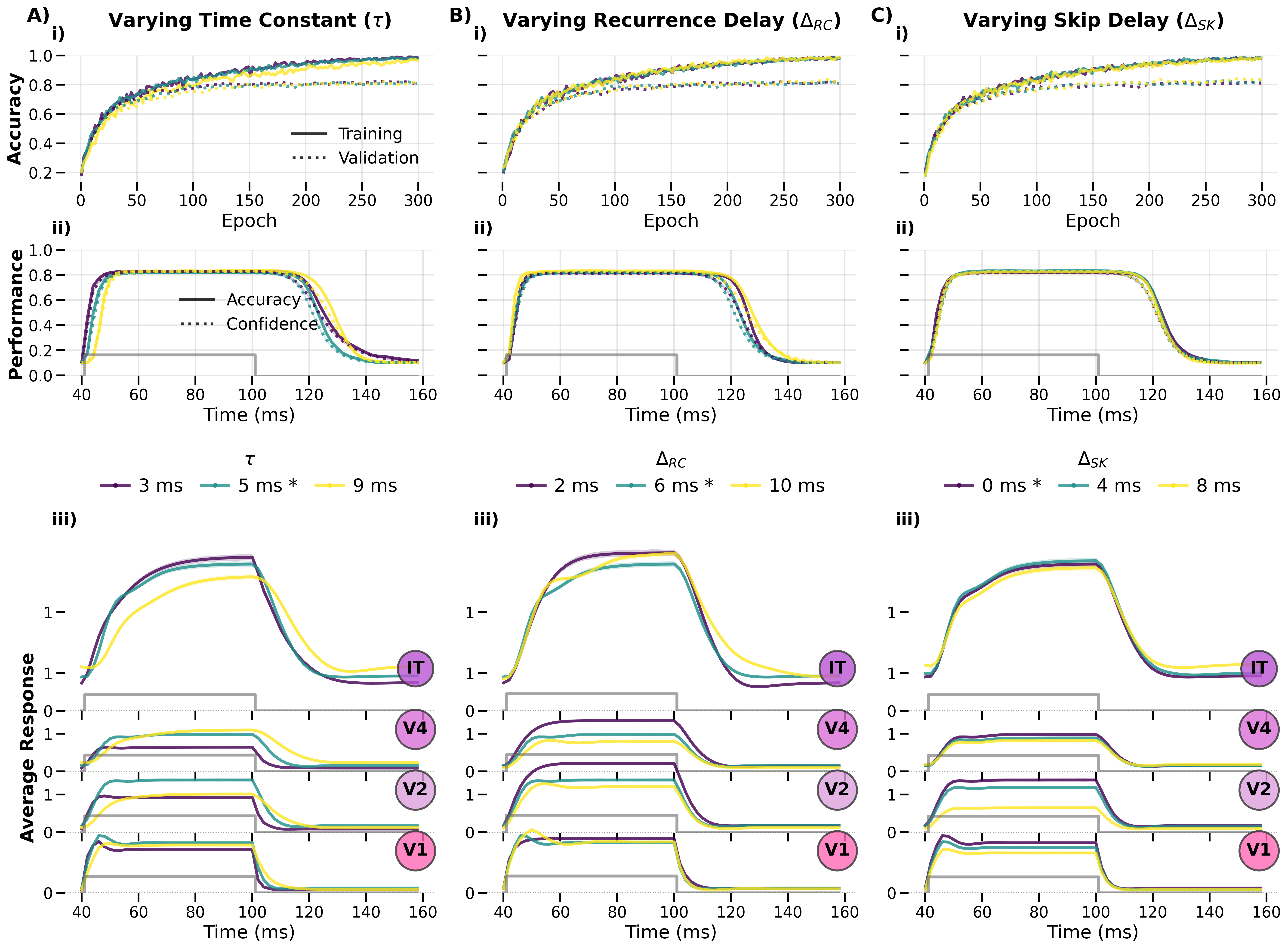
Figure: Per‑layer response trajectories across different time constants (τ) and recurrence delays (t_recurrence). The three‑panel layout isolates the contribution of each temporal parameter to the overall response shape.

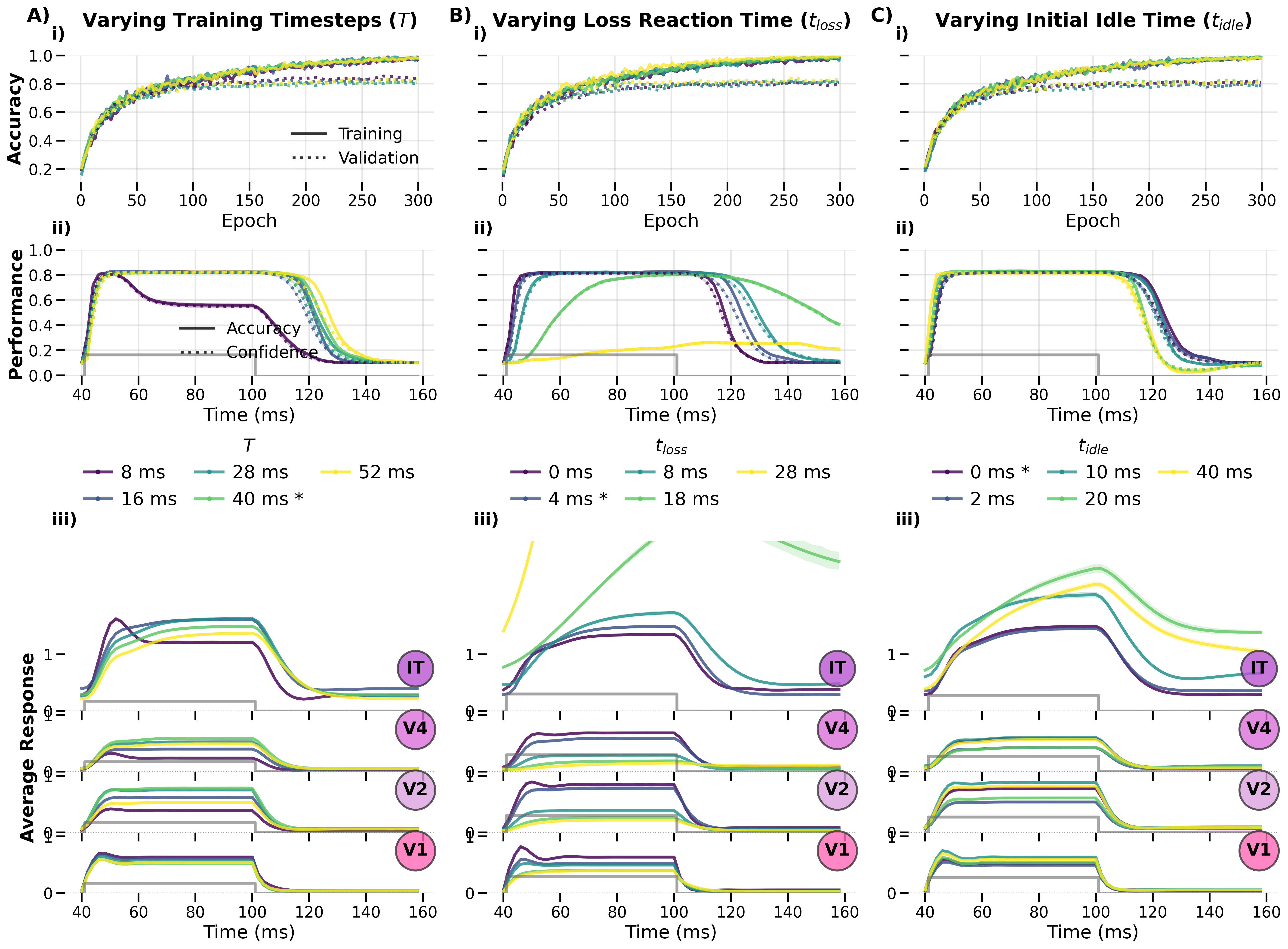
Figure: Response trajectories across varying numbers of timesteps and loss reaction‑time delays. The temporal window over which the loss is computed and the number of idle timesteps (no stimulus present) both shape the emergent dynamics.

Computational Considerations

Implementing continuous-time dynamics in neural networks poses several computational challenges:

Efficiency vs. Accuracy

There's a trade-off between computational efficiency and accuracy:

• Smaller time steps (dt) → Higher accuracy but more computation
• Larger time steps → Lower accuracy but faster computation

DynVision uses a default time step of 2ms, which provides a reasonable balance for most applications.

Memory Requirements

Storing neural states over time requires significant memory:

• Each layer needs to store its activation history
• History length depends on the longest delay (usually t_feedforward)
• Total memory scales with batch size × history length × layer size

DynVision implements several optimizations to manage memory usage:

• Efficient history management
• Optional CPU storage for responses
• Mixed precision computation

Gradient Propagation

Training models with temporal dynamics requires backpropagation through time, which:

• Creates large computational graphs
• Can lead to vanishing/exploding gradients
• Requires significant memory for intermediate activations

DynVision addresses these challenges with:

• Truncated backpropagation
• Gradient clipping
• Mixed precision training

Applications and Examples

The temporal dynamics in DynVision enable several interesting applications:

1. Modeling Perceptual Phenomena

Many perceptual phenomena involve temporal dynamics:

• Backward masking: When a briefly presented stimulus is masked by a subsequent stimulus
• Flash-lag effect: When a moving object appears ahead of a briefly flashed stationary object
• Motion perception: How the visual system integrates information over time to perceive motion

2. Studying Neurological Conditions

Altered temporal dynamics are associated with several neurological conditions:

• Autism: Altered excitation/inhibition balance affecting temporal integration
• Schizophrenia: Disrupted feedback processing
• Dyslexia: Deficits in rapid temporal processing

DynVision can be used to model these conditions by adjusting parameters like:

• Time constants
• Excitation/inhibition balance
• Feedback connection strength

3. Robust Object Recognition

Temporal processing may enhance object recognition:

• Disambiguation: Resolving ambiguous inputs through recurrent processing
• Noise reduction: Integrating information over time to reduce noise
• Occlusion handling: Completing partially occluded objects through feedback

4. Attention Mechanisms

Temporal dynamics play a crucial role in attention:

• Temporal selection: Enhancing processing at specific time points
• Rhythmic attention: Fluctuations in attentional processing
• Feature binding: Synchronization of neural activity

Future Directions

The implementation of temporal dynamics in DynVision opens several avenues for future research:

1. Oscillatory Dynamics

Adding oscillatory components to the neural dynamics could capture:

• Alpha/beta/gamma rhythms
• Phase-dependent processing
• Cross-frequency coupling

2. Heterogeneous Time Constants

Implementing cell-type specific time constants could model:

• Fast-spiking interneurons
• Regular-spiking pyramidal cells
• Intrinsically bursting neurons

3. Neuromodulation

Adding neuromodulatory influences could capture:

• Arousal-dependent processing
• Task-dependent dynamics
• Learning-dependent changes in temporal processing

4. Spike-Based Implementation

Moving towards spiking neural networks could provide:

• Greater biological realism
• Enhanced temporal precision
• Energy-efficient computation

Conclusion

Temporal dynamics are a fundamental aspect of biological visual processing that standard deep learning models often neglect. By implementing continuous-time dynamics with biologically motivated parameters, DynVision provides a framework for building more biologically plausible models of vision.

These models not only better capture the temporal properties of biological vision but also provide insights into how recurrent processing shapes visual perception. As computational resources continue to improve, incorporating these dynamics will become increasingly feasible and important for building truly brain-like artificial vision systems.

References

1. Groen, I. I. A., et al. (2022). Temporal Dynamics of Neural Responses in Human Visual Cortex.
2. Kietzmann, T. C., et al. (2019). Recurrence is required to capture the representational dynamics of the human visual system.
3. Kar, K., et al. (2019). Evidence that recurrent circuits are critical to the ventral stream's execution of core object recognition behavior.
4. Heeger, D. J., & Mackey, W. E. (2019). Oscillatory recurrent gated neural integrator circuits (ORGaNICs), a unifying theoretical framework for neural dynamics.
5. Soo, W. W., et al. (2024). Recurrent neural network dynamical systems for biological vision.