📗 Explanation · understanding-oriented
Engineering vs. Biological Time
This explanation covers the two time‑unrolling conventions in DynVision, their mathematical equivalence, and how to convert between them.
Two Ways of Unrolling
Biological time — each feedforward connection has a propagation delay (\(\Delta_{FF} > 0\)), so activity propagates through the network depth over multiple timesteps. This matches cortical conduction velocities.
Engineering time — set \(\Delta_{FF} = 0\) so that activity propagates from input to output within a single timestep. The network becomes computationally more efficient but the temporal graph is mathematically equivalent when delays are converted correctly.
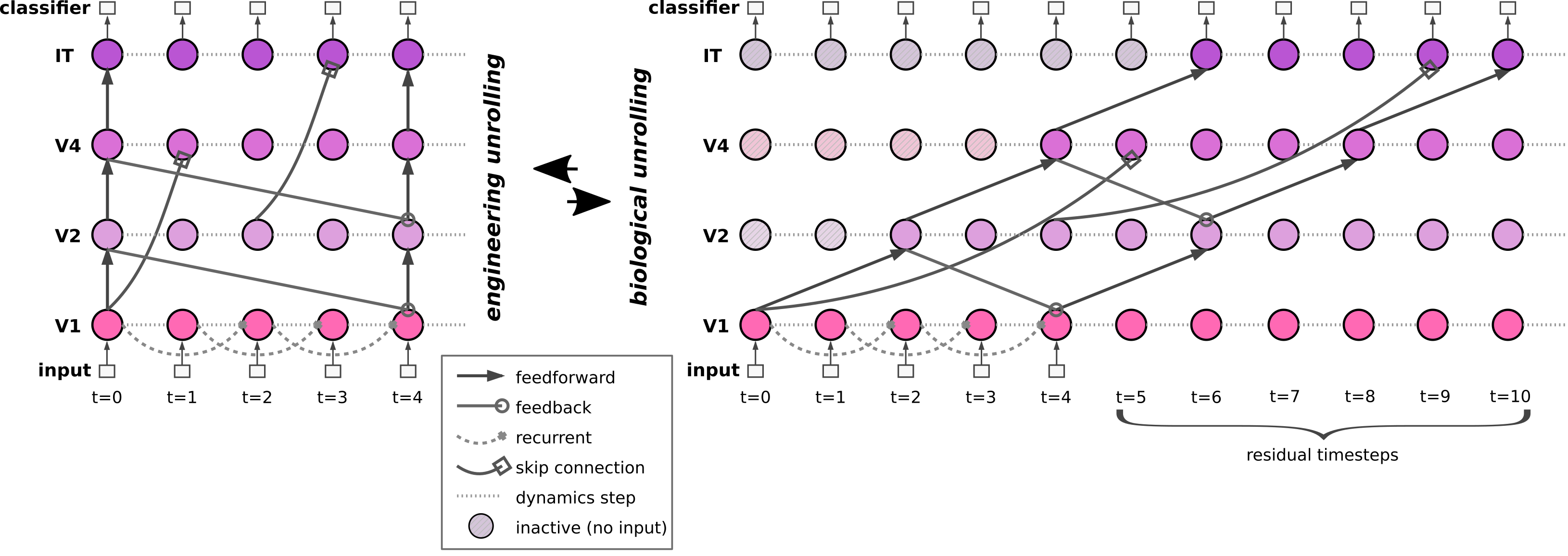
Figure: The same recurrent network unrolled in engineering time (left, \(\Delta_{FF}=0\)) and biological time (right, \(\Delta_{FF}=2\)). Signal flow through the network and time is identical in both conventions.
Delay Conversion Formulas
To switch from biological to engineering time in a network with skip and feedback connections:
where \(dL\) is the number of layers spanned by the connection.
Engineering‑time unrolling only works while \(\Delta_{SK}^{eng}\) is positive — i.e. skip connections must be as fast as, or faster than, the multi‑synaptic feedforward pathway.
Note: In practice these formulas may need a \(\pm 1\) offset depending on the order of operations. Skip delays typically need an increment because the source layer's computation for the current timestep has already been executed; feedback source computations for the same timestep have not.
Example
A DyRCNNx8 with full recurrence trained on CIFAR‑100 (30 timesteps, \(dt = 2\) ms):
| Parameter | Engineering | Biological |
|---|---|---|
| \(\Delta_{FF}\) | 0 ms | 10 ms |
| \(\Delta_{RC}\) | 6 ms | 6 ms |
| \(\Delta_{SK}\) | 2 ms | 22 ms |
| \(\Delta_{FB}\) | 30 ms | 10 ms |
Training in engineering time decreases epoch time by ~29 % and GPU memory from 2.39 GB to 2.13 GB.
Equivalence Validation
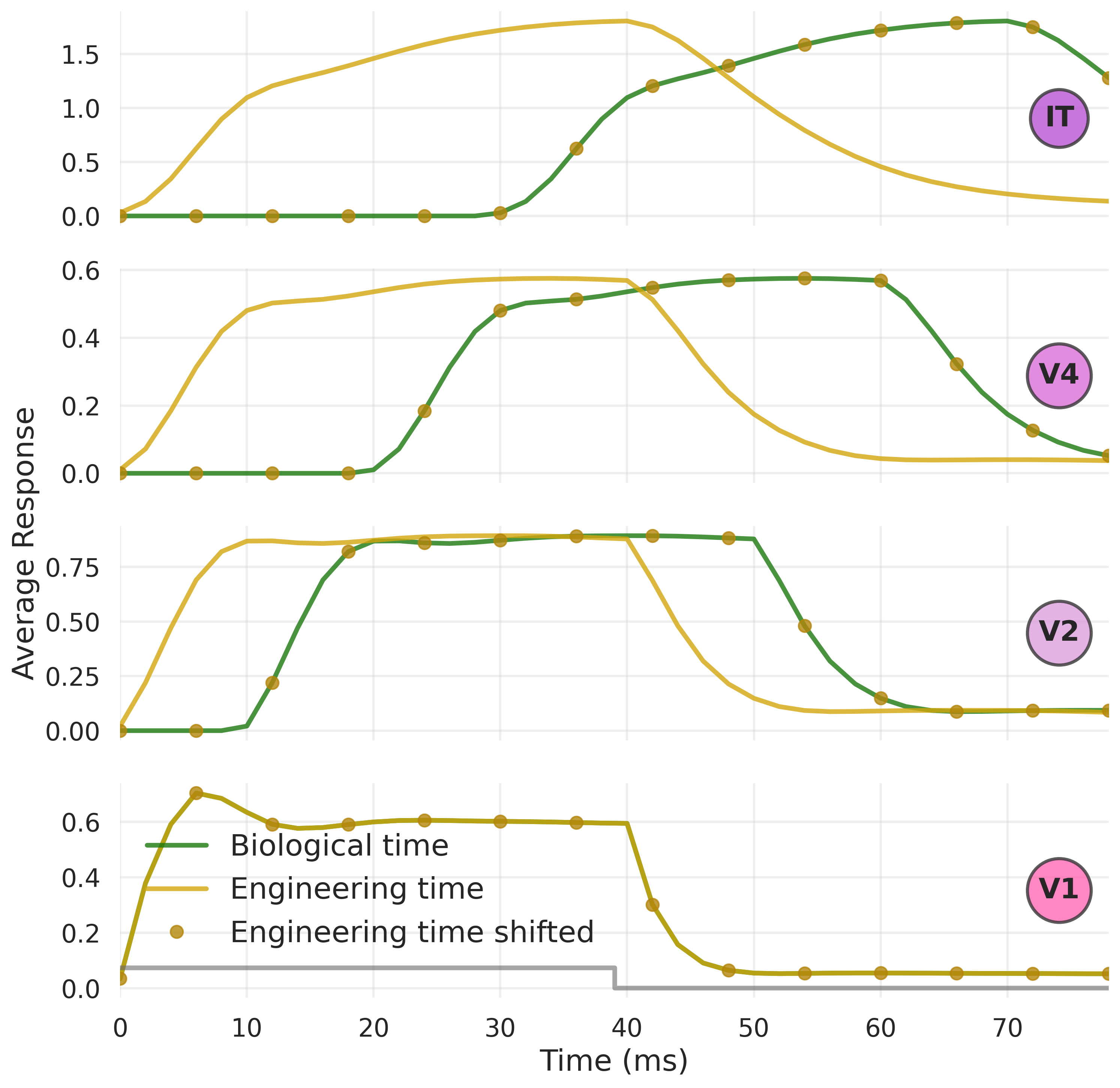
Figure: A DyRCNNx8 model trained in engineering time (with skip and feedback) and tested in both conventions produces identical temporal dynamics (shifted by \(\Delta_{FF}\)). This confirms that researchers can use the computationally more efficient engineering time for training while interpreting results in biological time.
The recurrence delay (\(\Delta_{RC} = 6\) ms) and time constant (\(\tau = 5\) ms) are independent of the unrolling convention; only the feedforward delay distinguishes them.
See Also
- Temporal Dynamics — dynamical systems formulation
- Dynamics Solvers — ODE solver reference
- Benchmarking — computational cost comparison