📗 Explanation · understanding-oriented

Comparison to Neural Data¶

This explanation summarises how DynVision model responses compare to electrophysiological recordings and human behavioural data.

Approach¶

We compare model dynamics to real neural data using methods inspired by neural data analysis. Following Groen et al. (2022), we test whether models exhibit temporally delayed normalisation: adaptation to repeated stimuli, sublinear summation to stimuli of increasing duration, and contrast‑dependent reaction time.

As an analogue of ECoG broadband power, we average model activations per layer and timestep. The temporal presentation pattern 1011 (shuffled) is used during training to improve null‑response behaviour.

Temporal Normalisation Without Explicit Normalisation¶

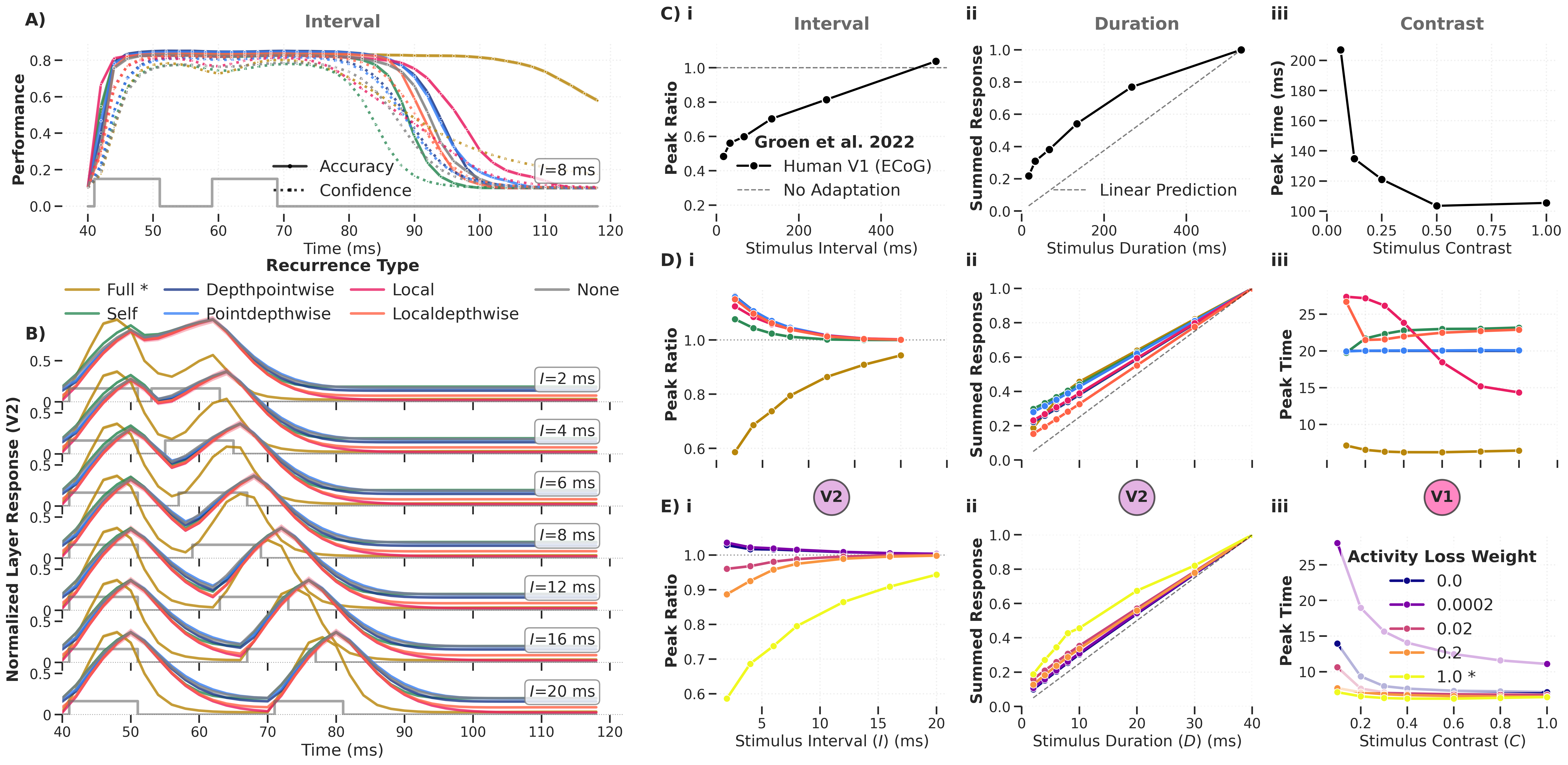
Temporal dynamics by recurrence type (V2)

Figure: Temporal dynamics of the DyRCNNx8 model for different recurrence types, tested on varied inter‑stimulus interval (i), stimulus duration (ii), and contrast (iii). Panel C shows experimental ECoG data from Groen et al. (2022); panels D and E show the corresponding characteristics in model variants.

Key findings:

Adaptation (reduced response to repeated stimuli, peak ratio < 1) emerges only for full recurrence with large activity‑loss weights. Other recurrence types show the opposite: the second peak is larger than the first.
Sublinear summation is also most pronounced for full recurrence with strong activity loss.
Contrast‑dependent reaction time appears for local recurrence or for full recurrence with minimal activity loss — the opposite condition to adaptation and summation.

The model architecture contains no explicit normalisation operation. Any normalisation effect relies entirely on recurrent connections — demonstrating that continuous‑time recurrent dynamics can naturally produce cortical temporal phenomena.

Two Functionally Distinct Regimes¶

These results reveal a dissociation between two dynamic regimes:

Regime	Configuration	Phenomena
Temporal normalisation	Full recurrence, output target, strong activity loss	Adaptation, sublinear summation
Noise robustness	Full recurrence, middle target, minimal activity loss	Human‑level noise robustness, contrast‑dependent RT

Noise Robustness vs. Humans¶

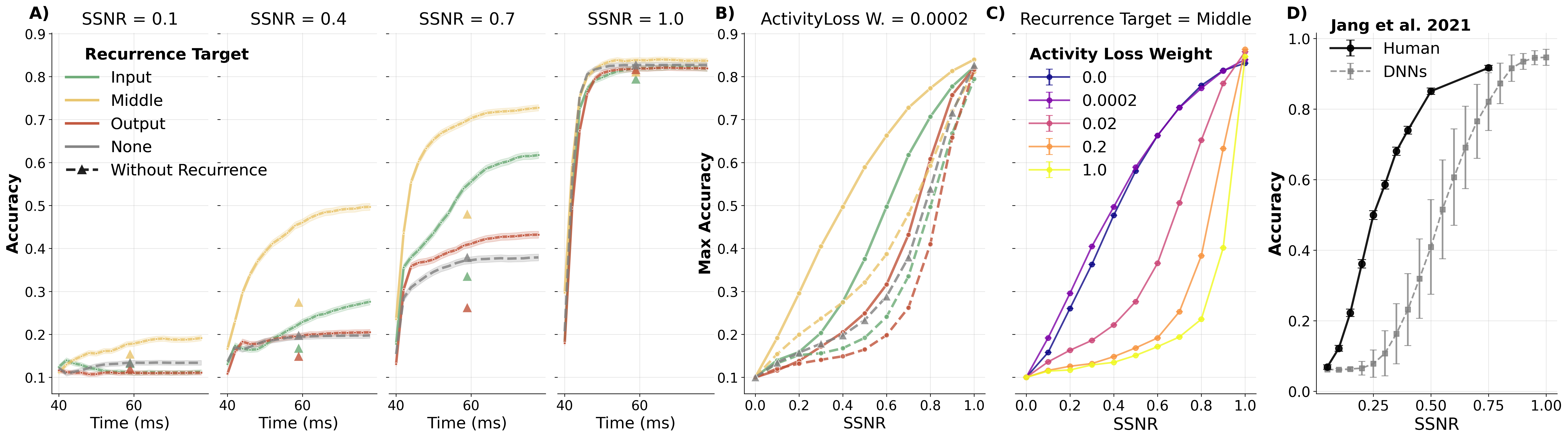
Noise robustness by recurrence target

Figure: Noise robustness depends on where the recurrent signal is integrated (input, middle, or output). The middle‑target variant best captures human performance trends (panel D, Jang et al. 2021). Disabling recurrence at test time (△ markers) confirms that robustness comes from active temporal integration, not static architecture.

Higher activity‑loss weights reduce noise robustness, creating an unexpected trade‑off: the same constraint that promotes biologically realistic normalisation also degrades robustness.

Supplementary Results¶

Additional comparisons are available for:

V1 vs V2 layer responses across recurrence types and targets (triggering complementary results where V1 responses to contrast experiments better match the data).
Feedback connections — no systematic noise‑robustness benefit across seeds.
Different recurrence types at matched noise‑robustness conditions.

Temporal dynamics (V1/V2 swapped)

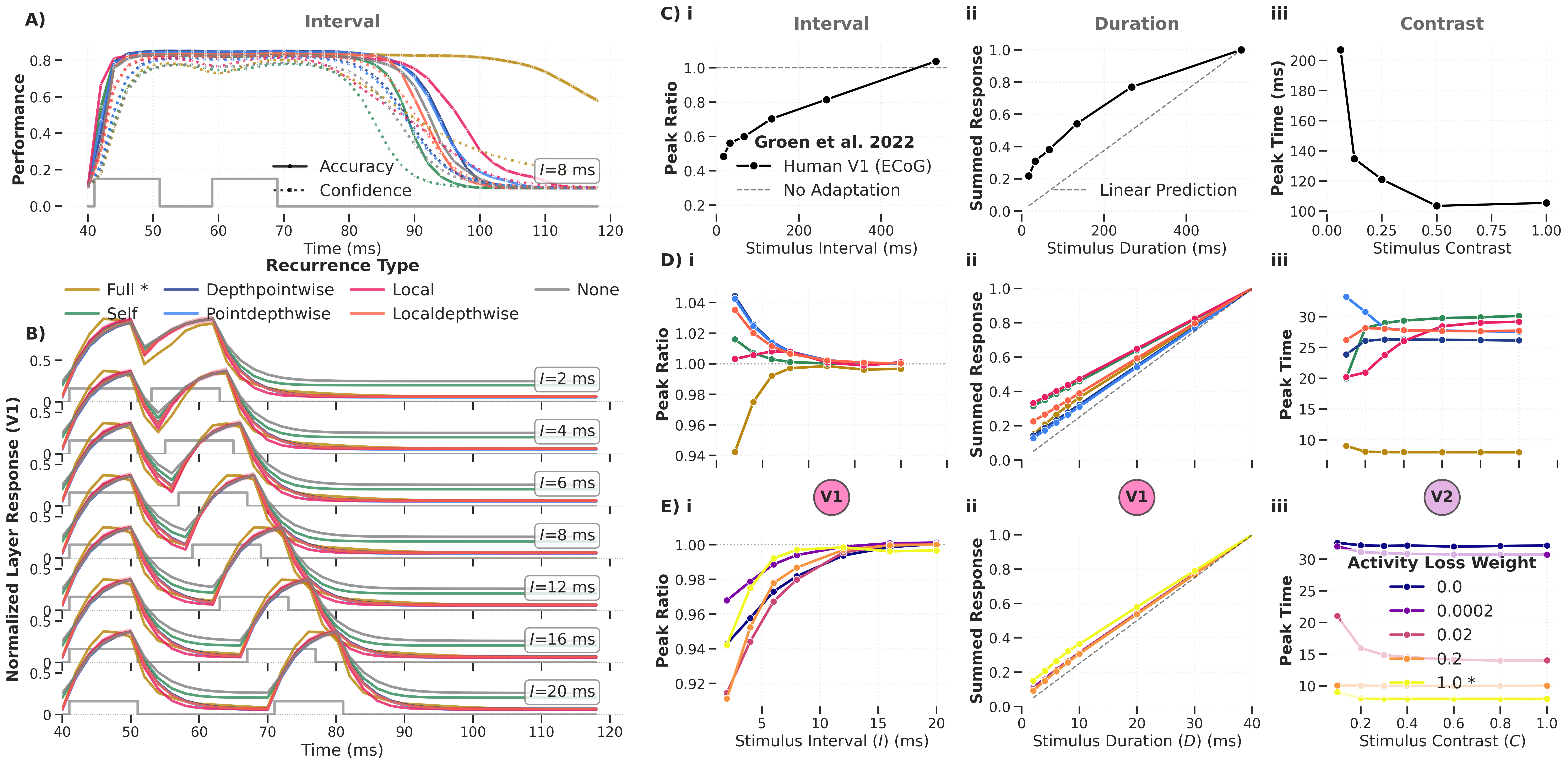
Figure: Same analysis with V1 and V2 layer summaries swapped, showing that V1 responses to contrast experiments better match the Groen et al. reference data.

Recurrence Target Analysis¶

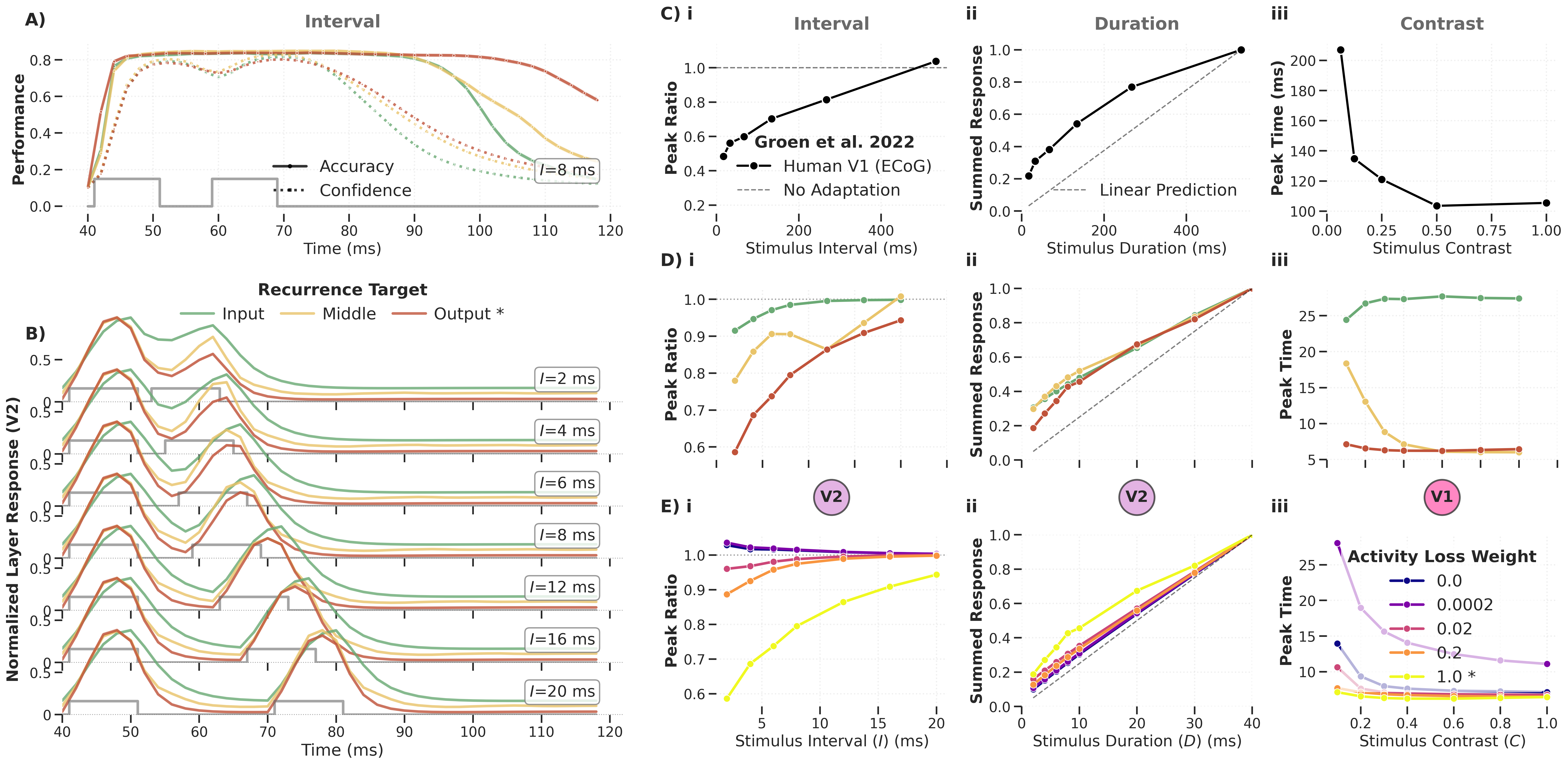
Temporal dynamics by recurrence target (V2)

Figure: Temporal dynamics analysis of the DyRCNNx8 model across recurrence targets (input, middle, output). The target position qualitatively changes which temporal phenomena emerge.

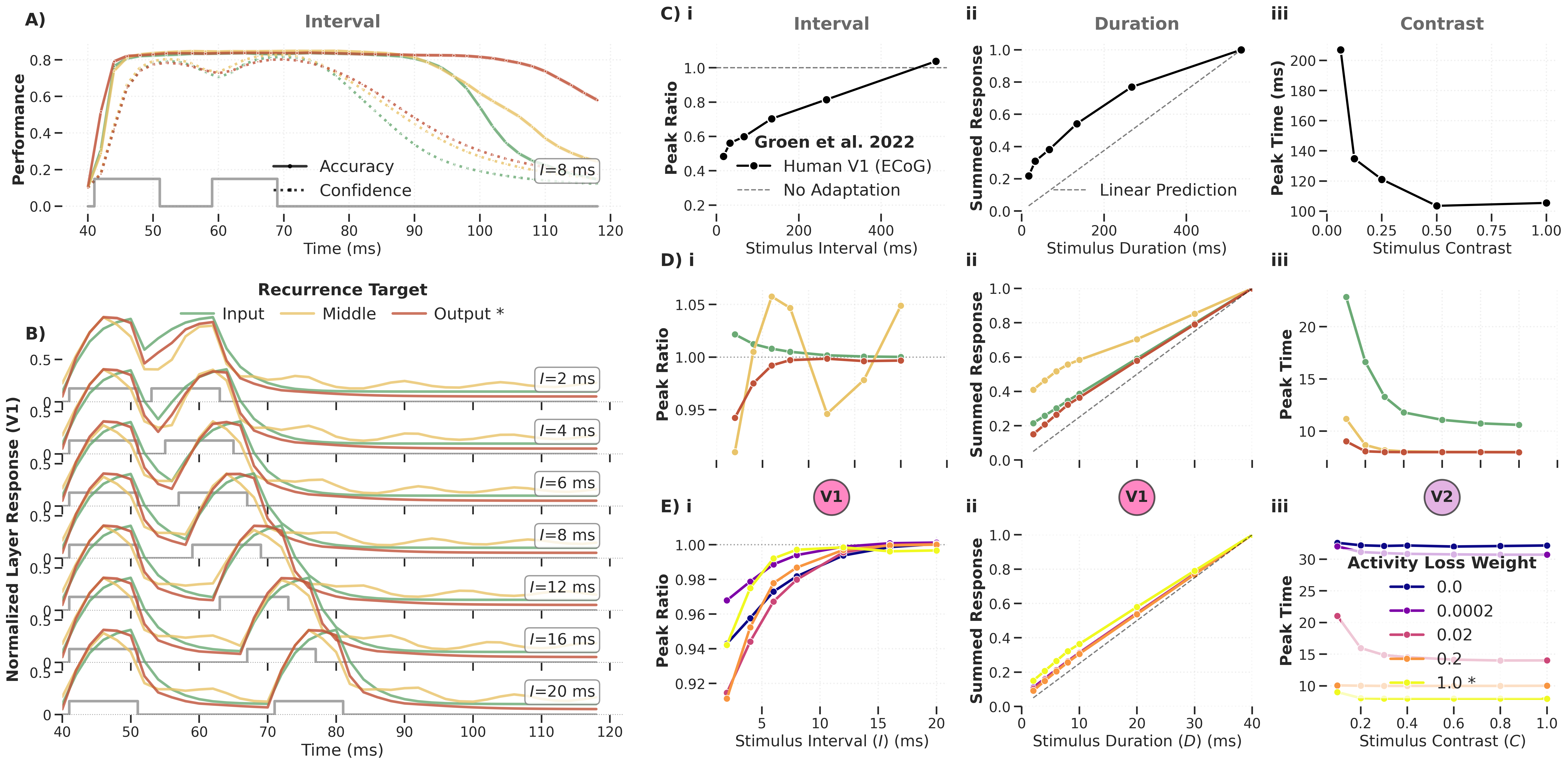
Temporal dynamics by recurrence target (V1/V2 swapped)

Figure: Same recurrence‑target analysis with V1 and V2 layer summaries swapped.

Training and Stability¶

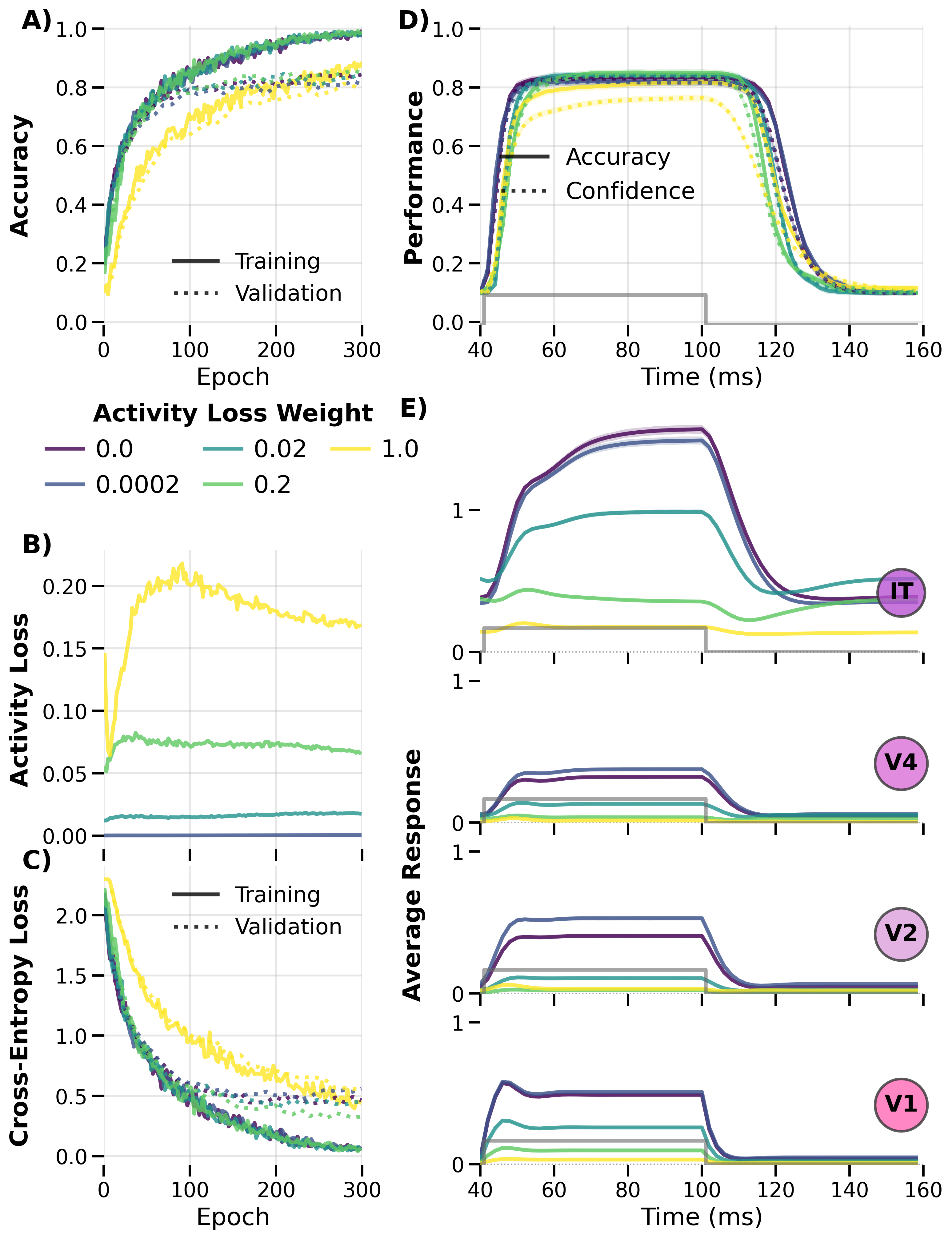
Training dynamics with activity loss

Figure: Training dynamics across activity‑loss weights showing convergence properties and the trade‑off between regularization strength and final accuracy. The 1 presentation pattern is used here.

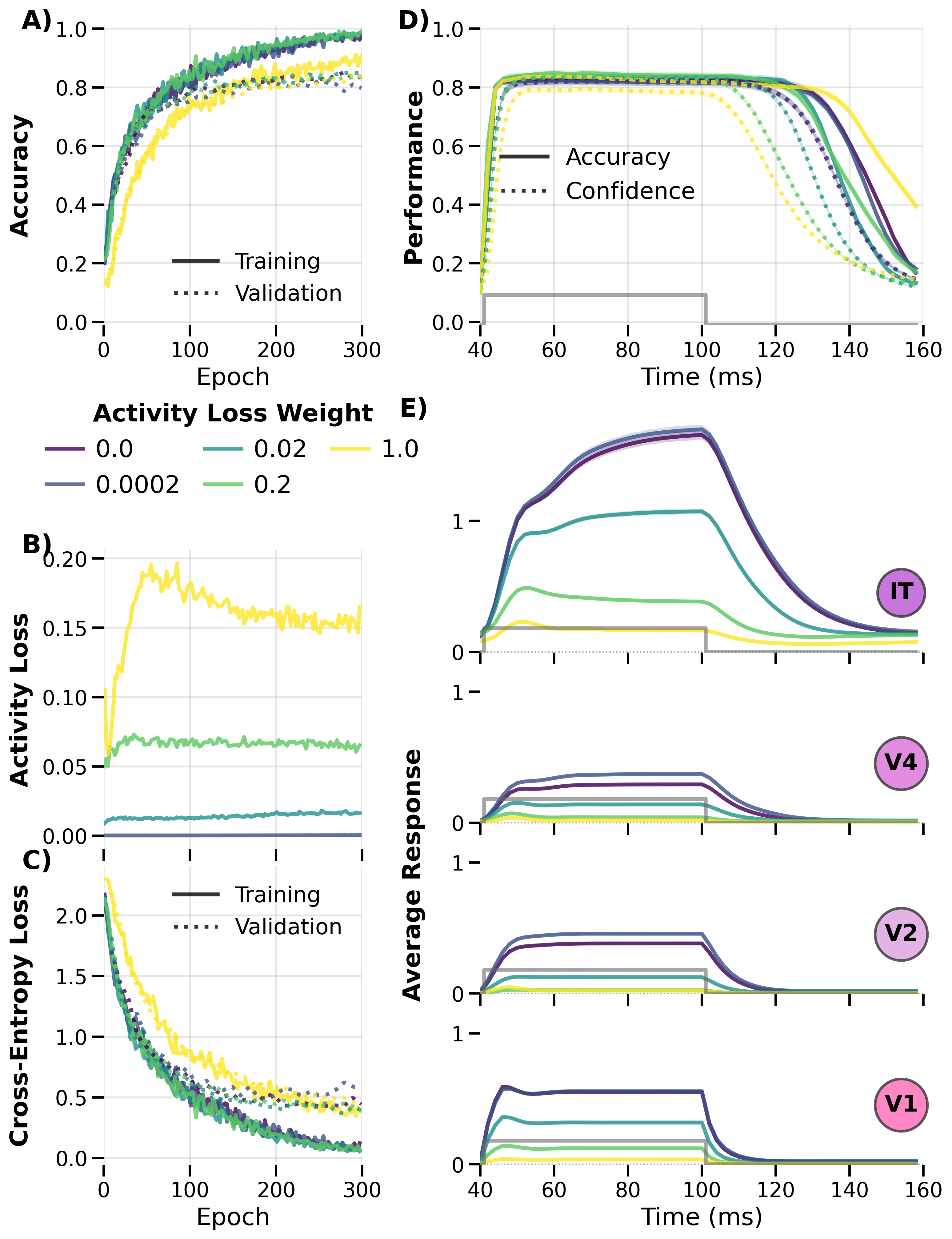
Training dynamics with alternating pattern

Figure: Same training‑dynamics analysis with the 1011 alternating presentation pattern. The pattern choice affects convergence speed but not the qualitative regularization trade‑off.

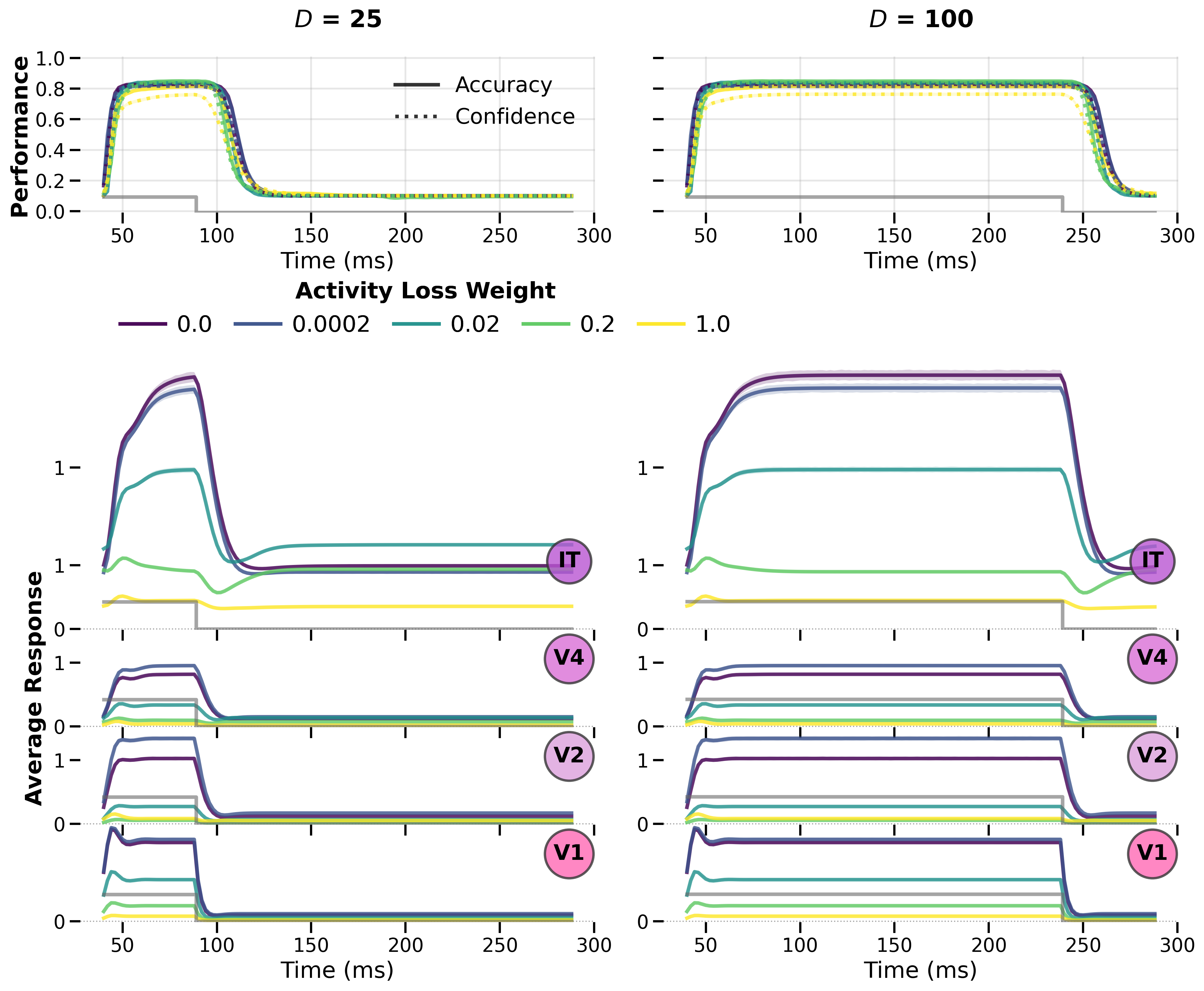
Stability analysis with activity loss

Figure: Parameter stability analysis across activity‑loss weights. The map reveals regions of stable convergence vs. regions where the dynamics become unstable, explaining why certain configurations fail to train.

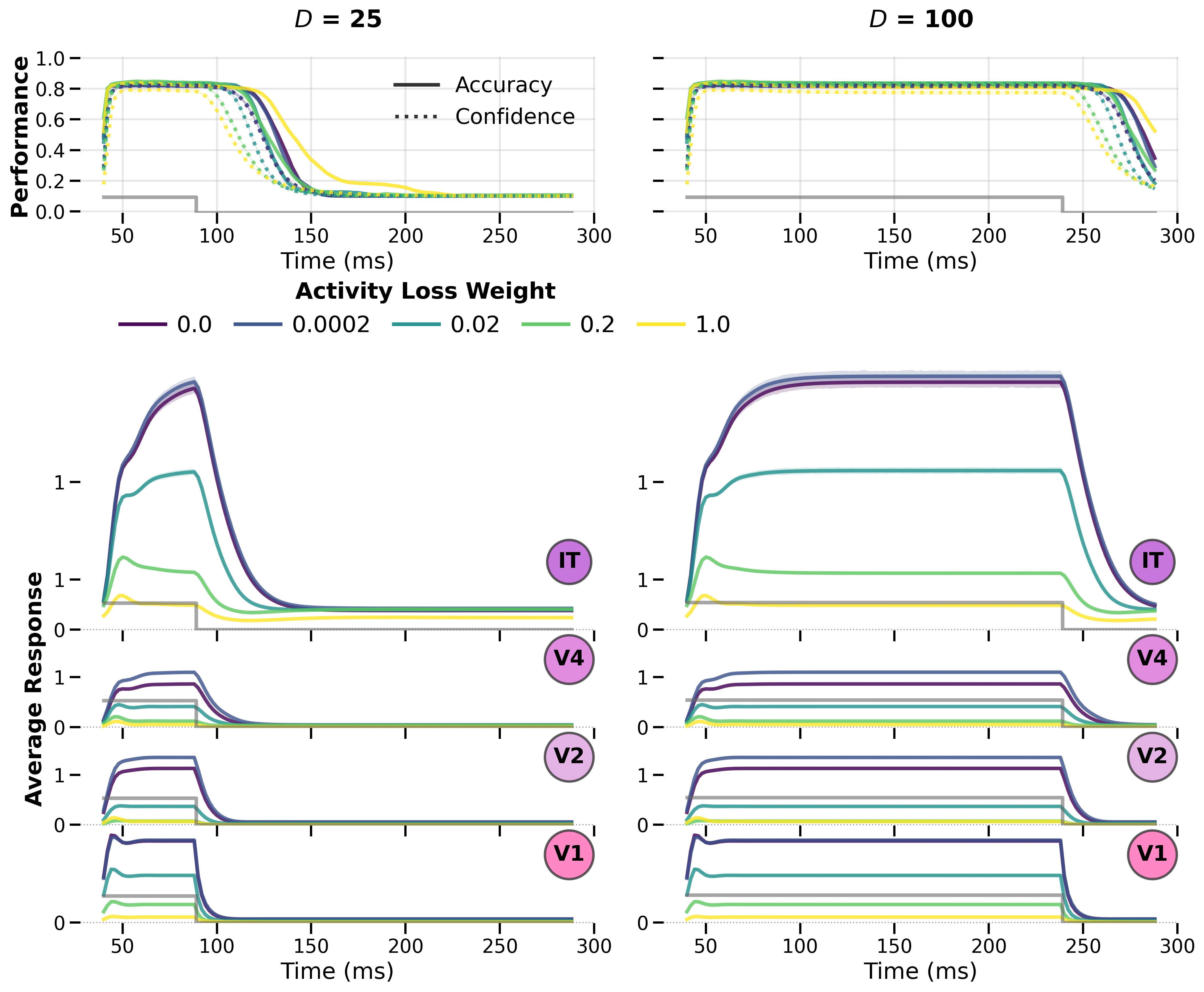
Stability analysis with alternating pattern

Figure: Same stability analysis with the 1011 pattern, confirming that the instability regions are consistent across presentation patterns.

References¶

Groen, I. I. A., et al. (2022). Temporal Dynamics of Neural Responses in Human Visual Cortex.
Jang, H., et al. (2021). Noise‑trained deep neural networks effectively predict human vision in a crowded task.
Heeger, D. J., & Mackey, W. E. (2019). ORGaNICs.
Rubin, D. B., et al. (2015). The stabilized supralinear network.